

Which Regression Equation Best Fits These Data Brainly
Affiliate 7: Correlation and Simple Linear Regression
In many studies, we measure out more than than i variable for each individual. For example, nosotros measure precipitation and plant growth, or number of young with nesting habitat, or soil erosion and volume of h2o. Nosotros collect pairs of data and instead of examining each variable separately (univariate data), we want to find ways to describe bivariate data, in which two variables are measured on each subject in our sample. Given such data, nosotros begin by determining if there is a relationship between these two variables. Every bit the values of one variable change, do we run into respective changes in the other variable?
We tin depict the human relationship between these 2 variables graphically and numerically. Nosotros begin past considering the concept of correlation.
Correlation is divers every bit the statistical association between two variables.
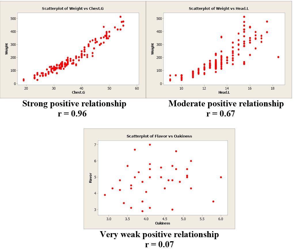
A correlation exists between two variables when ane of them is related to the other in some fashion. A scatterplot is the best place to start. A scatterplot (or besprinkle diagram) is a graph of the paired (x, y) sample data with a horizontal x-centrality and a vertical y-axis. Each individual (x, y) pair is plotted as a unmarried betoken.
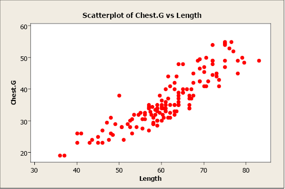
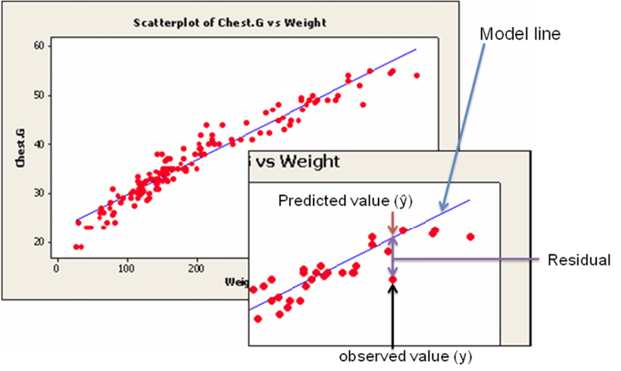
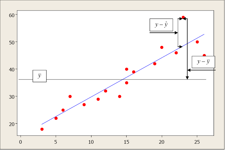
In this example, we plot comport chest girth (y) confronting bear length (x). When examining a scatterplot, we should study the overall blueprint of the plotted points. In this case, we run into that the value for breast girth does tend to increment as the value of length increases. Nosotros can see an upwards slope and a direct-line blueprint in the plotted data points.
A scatterplot can identify several unlike types of relationships between two variables.
- A relationship has no correlation when the points on a scatterplot practice non bear witness whatever blueprint.
- A relationship is non-linear when the points on a scatterplot follow a blueprint simply not a straight line.
- A relationship is linear when the points on a scatterplot follow a somewhat straight line design. This is the human relationship that nosotros will examine.
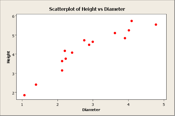
Linear relationships can be either positive or negative. Positive relationships have points that incline upward to the right. As 10 values increment, y values increase. As x values decrease, y values decrease. For case, when studying plants, elevation typically increases as diameter increases.
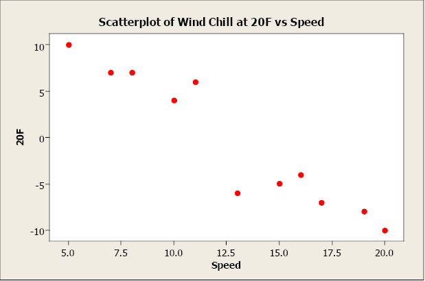
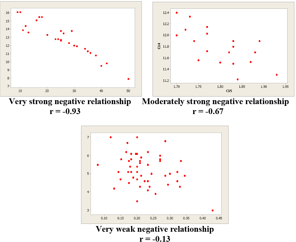
Negative relationships have points that decline downward to the right. As 10 values increase, y values subtract. As x values decrease, y values increase. For example, as wind speed increases, wind chill temperature decreases.
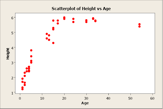
Non-linear relationships have an credible design, just not linear. For instance, as age increases elevation increases up to a signal then levels off subsequently reaching a maximum height.
When ii variables take no relationship, there is no straight-line relationship or non-linear relationship. When i variable changes, it does non influence the other variable.
Linear Correlation Coefficient
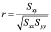
Because visual examinations are largely subjective, nosotros need a more precise and objective mensurate to define the correlation between the ii variables. To quantify the forcefulness and direction of the relationship between two variables, we use the linear correlation coefficient:
where x̄ and s10 are the sample mean and sample standard deviation of the 10's, and ȳ and sy are the mean and standard difference of the y's. The sample size is due north.
An alternating ciphering of the correlation coefficient is:
where 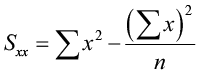
The linear correlation coefficient is too referred to as Pearson's product moment correlation coefficient in honour of Karl Pearson, who originally developed it. This statistic numerically describes how strong the straight-line or linear relationship is between the ii variables and the management, positive or negative.
The properties of "r":
- It is always between -i and +1.
- It is a unitless mensurate so "r" would be the same value whether you measured the two variables in pounds and inches or in grams and centimeters.
- Positive values of "r" are associated with positive relationships.
- Negative values of "r" are associated with negative relationships.
Examples of Positive Correlation
Examples of Negative Correlation
Correlation is not causation!!! Just considering two variables are correlated does not mean that one variable causes another variable to change.
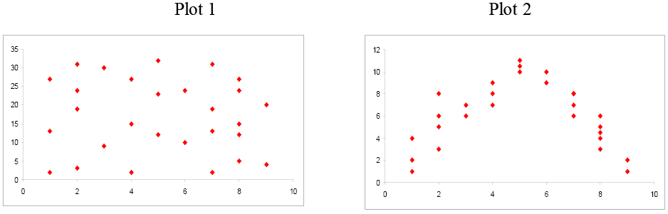
Examine these side by side two scatterplots. Both of these data sets have an r = 0.01, but they are very different. Plot 1 shows piddling linear human relationship between x and y variables. Plot 2 shows a strong non-linear relationship. Pearson'due south linear correlation coefficient simply measures the strength and direction of a linear relationship. Ignoring the scatterplot could consequence in a serious mistake when describing the relationship between ii variables.
When you investigate the relationship between 2 variables, e'er begin with a scatterplot. This graph allows y'all to look for patterns (both linear and non-linear). The adjacent stride is to quantitatively depict the force and direction of the linear relationship using "r". One time you have established that a linear relationship exists, you can take the next footstep in model building.
Simple Linear Regression
One time we take identified ii variables that are correlated, we would like to model this relationship. We want to use one variable every bit a predictor or explanatory variable to explain the other variable, the response or dependent variable. In club to practise this, we need a good human relationship betwixt our two variables. The model tin can then be used to predict changes in our response variable. A strong relationship between the predictor variable and the response variable leads to a expert model.
A simple linear regression model is a mathematical equation that allows usa to predict a response for a given predictor value.
Our model will take the form of ŷ = b 0 + b1ten where b 0 is the y-intercept, b i is the gradient, x is the predictor variable, and ŷ an gauge of the mean value of the response variable for whatever value of the predictor variable.
The y-intercept is the predicted value for the response (y) when x = 0. The slope describes the change in y for each one unit of measurement alter in ten. Allow'south look at this example to clarify the interpretation of the slope and intercept.
Instance 1
A hydrologist creates a model to predict the volume menses for a stream at a span crossing with a predictor variable of daily rainfall in inches.
ŷ = i.vi + 29x. The y-intercept of ane.6 can be interpreted this style: On a day with no rainfall, there volition be 1.6 gal. of h2o/min. flowing in the stream at that span crossing. The slope tells united states that if it rained ane inch that day the flow in the stream would increment past an additional 29 gal./min. If it rained 2 inches that day, the period would increment by an additional 58 gal./min.
Instance 2
What would be the average stream menses if it rained 0.45 inches that day?
ŷ = 1.6 + 29x = 1.6 + 29(0.45) = 14.65 gal./min.
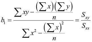
The To the lowest degree-Squares Regression Line (shortcut equations)
The equation is given past ŷ = b 0 + bone x
where  is the slope and b0 = ŷ – b1 x̄ is the y-intercept of the regression line.
An alternate computational equation for gradient is:
This simple model is the line of all-time fit for our sample data. The regression line does not get through every point; instead information technology balances the difference between all data points and the straight-line model. The difference between the observed data value and the predicted value (the value on the straight line) is the error or residual. The criterion to decide the line that best describes the relation between 2 variables is based on the residuals.
Rest = Observed – Predicted
For example, if yous wanted to predict the chest girth of a black comport given its weight, you could use the following model.
Chest girth = thirteen.ii +0.43 weight
The predicted breast girth of a bear that weighed 120 lb. is 64.8 in.
Chest girth = thirteen.ii + 0.43(120) = 64.8 in.
Merely a measured conduct chest girth (observed value) for a behave that weighed 120 lb. was really 62.1 in.
The residual would be 62.1 – 64.viii = -2.7 in.
A negative residual indicates that the model is over-predicting. A positive residue indicates that the model is under-predicting. In this instance, the model over-predicted the breast girth of a acquit that actually weighed 120 lb.
This random error (rest) takes into account all unpredictable and unknown factors that are not included in the model. An ordinary to the lowest degree squares regression line minimizes the sum of the squared errors betwixt the observed and predicted values to create a best plumbing equipment line. The differences between the observed and predicted values are squared to bargain with the positive and negative differences.
Coefficient of Determination
Later we fit our regression line (compute b 0 and b one), nosotros usually wish to know how well the model fits our data. To determine this, nosotros need to think back to the idea of analysis of variance. In ANOVA, we partitioned the variation using sums of squares so we could identify a handling result opposed to random variation that occurred in our data. The thought is the aforementioned for regression. We want to partition the total variability into 2 parts: the variation due to the regression and the variation due to random fault. And nosotros are again going to compute sums of squares to assist the states do this.
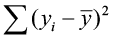
Suppose the total variability in the sample measurements most the sample mean is denoted by 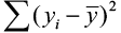 , called the sums of squares of full variability nearly the mean (SST). The squared difference between the predicted value
  and the sample hateful is denoted past
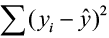
 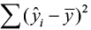 , called the sums of squares due to regression (SSR). The SSR represents the variability explained past the regression line. Finally, the variability which cannot be explained by the regression line is called the sums of squares due to mistake (SSE) and is denoted past
 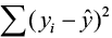 . SSE is actually the squared residual.
| SST | = SSR | + SSE |
| | = | + |

The sums of squares and mean sums of squares (but like ANOVA) are typically presented in the regression analysis of variance tabular array. The ratio of the hateful sums of squares for the regression (MSR) and hateful sums of squares for error (MSE) form an F-test statistic used to test the regression model.
The relationship betwixt these sums of square is defined as
Full Variation = Explained Variation + Unexplained Variation
The larger the explained variation, the better the model is at prediction. The larger the unexplained variation, the worse the model is at prediction. A quantitative measure of the explanatory power of a model is R2, the Coefficient of Decision:
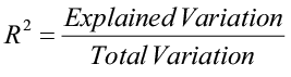
The Coefficient of Determination measures the pct variation in the response variable (y) that is explained by the model.
- Values range from 0 to one.
- An R2 shut to zero indicates a model with very little explanatory power.
- An R2 close to one indicates a model with more than explanatory ability.
The Coefficient of Decision and the linear correlation coefficient are related mathematically.
R2 = rtwo
Nonetheless, they accept two very different meanings: r is a measure of the forcefulness and management of a linear relationship between two variables; R 2 describes the percent variation in "y" that is explained by the model.
Residual and Normal Probability Plots
Fifty-fifty though you have determined, using a scatterplot, correlation coefficient and Rtwo, that x is useful in predicting the value of y, the results of a regression analysis are valid only when the data satisfy the necessary regression assumptions.
- The response variable (y) is a random variable while the predictor variable (x) is assumed non-random or fixed and measured without error.
- The relationship between y and x must be linear, given by the model
 .
. - The mistake of random term the values ε are independent, have a mean of 0 and a common variance σ ii, independent of x, and are commonly distributed.
We can apply residuum plots to cheque for a constant variance, besides as to make sure that the linear model is in fact adequate. A residual plot is a scatterplot of the residue (= observed – predicted values) versus the predicted or fitted (as used in the balance plot) value. The center horizontal centrality is set up at zero. One belongings of the residuals is that they sum to null and have a mean of nothing. A residual plot should be free of any patterns and the residuals should appear every bit a random scatter of points about nada.
A residual plot with no appearance of any patterns indicates that the model assumptions are satisfied for these information.
A rest plot that has a "fan shape" indicates a heterogeneous variance (non-constant variance). The residuals tend to fan out or fan in as mistake variance increases or decreases.
A residual plot that tends to "swoop" indicates that a linear model may not exist advisable. The model may demand higher-order terms of ten, or a non-linear model may exist needed to better describe the relationship between y and x. Transformations on ten or y may also exist considered.
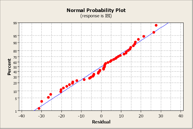
A normal probability plot allows us to check that the errors are normally distributed. It plots the residuals confronting the expected value of the residual every bit if information technology had come from a normal distribution. Call up that when the residuals are commonly distributed, they will follow a straight-line design, sloping upward.
This plot is not unusual and does not bespeak any not-normality with the residuals.
This next plot conspicuously illustrates a non-normal distribution of the residuals.
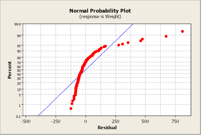
The near serious violations of normality commonly appear in the tails of the distribution because this is where the normal distribution differs most from other types of distributions with a similar mean and spread. Curvature in either or both ends of a normal probability plot is indicative of nonnormality.
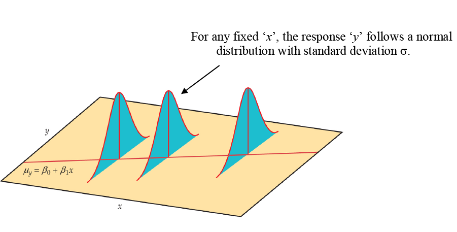
Population Model
Our regression model is based on a sample of n bivariate observations drawn from a larger population of measurements.
Nosotros use the means and standard deviations of our sample data to compute the gradient (b ane) and y-intercept (b 0) in guild to create an ordinary least-squares regression line. But we want to draw the human relationship betwixt y and x in the population, non merely within our sample information. We want to construct a population model. Now we will call up of the least-squares line computed from a sample as an approximate of the true regression line for the population.
The Population Model
 , where μ y is the population mean response, β 0 is the y-intercept, and β 1 is the slope for the population model.
In our population, there could be many different responses for a value of 10. In simple linear regression, the model assumes that for each value of 10 the observed values of the response variable y are normally distributed with a hateful that depends on x. Nosotros use μ y to represent these means. We also assume that these means all lie on a straight line when plotted against x (a line of means).
The sample data then fit the statistical model:
Information = fit + residual
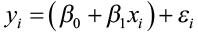
where the errors (ε i) are independent and normally distributed N (0, σ). Linear regression likewise assumes equal variance of y (σ is the same for all values of x). We utilise ε (Greek epsilon) to correspond the residual part of the statistical model. A response y is the sum of its mean and gamble deviation ε from the mean. The deviations ε represents the "noise" in the information. In other words, the noise is the variation in y due to other causes that preclude the observed (x, y) from forming a perfectly straight line.
The sample data used for regression are the observed values of y and x. The response y to a given x is a random variable, and the regression model describes the mean and standard departure of this random variable y. The intercept β 0, slope β i, and standard divergence σ of y are the unknown parameters of the regression model and must be estimated from the sample data.
ŷ is an unbiased guess for the mean response μ y
b 0 is an unbiased estimate for the intercept β 0
b 1 is an unbiased estimate for the slope β 1
Parameter Estimation
Once we have estimates of β 0 and β 1 (from our sample data b 0 and b i), the linear relationship determines the estimates of μ y for all values of x in our population, non just for the observed values of x. Nosotros now desire to utilize the least-squares line as a basis for inference almost a population from which our sample was fatigued.
Model assumptions tell usa that b 0 and b 1 are normally distributed with means β 0 and β 1 with standard deviations that can be estimated from the data. Procedures for inference about the population regression line will be similar to those described in the previous affiliate for means. As always, it is important to examine the data for outliers and influential observations.
In club to practice this, we need to estimate σ, the regression standard fault. This is the standard deviation of the model errors. It measures the variation of y about the population regression line. We will apply the residuals to compute this value. Call back, the predicted value of y ( p̂ ) for a specific x is the point on the regression line. Information technology is the unbiased judge of the mean response (μ y) for that x. The residual is:
residual = observed – predicted
due east i = y i – ŷ = 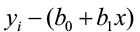
The rest due east i corresponds to model deviation ε i where Σ e i = 0 with a mean of 0. The regression standard error southward is an unbiased estimate of σ.
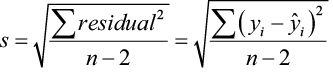
The quantity s is the judge of the regression standard fault (σ) and s 2 is ofttimes chosen the mean square error (MSE). A small value of s suggests that observed values of y fall shut to the true regression line and the line  should provide accurate estimates and predictions.
Confidence Intervals and Significance Tests for Model Parameters
In an earlier chapter, we synthetic conviction intervals and did significance tests for the population parameter μ (the population mean). We relied on sample statistics such as the mean and standard deviation for bespeak estimates, margins of errors, and test statistics. Inference for the population parameters β 0 (gradient) and β 1 (y-intercept) is very similar.
Inference for the slope and intercept are based on the normal distribution using the estimates b 0 and b 1. The standard deviations of these estimates are multiples of σ, the population regression standard error. Recollect, nosotros judge σ with south (the variability of the information well-nigh the regression line). Because we use south, we rely on the student t-distribution with (n – 2) degrees of freedom.
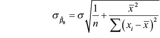
The standard error for judge of β 0
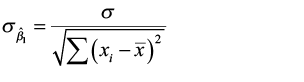
The standard error for gauge of β one
We can construct conviction intervals for the regression slope and intercept in much the aforementioned style as nosotros did when estimating the population mean.
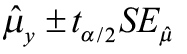
A confidence interval for β 0 : b 0 ± t α /2 SEb0
A confidence interval for β 1 : b 1 ± t α /2 SEb1
where SEb0 and SEb1 are the standard errors for the y-intercept and gradient, respectively.
Nosotros can also test the hypothesis H0: β 1 = 0. When we substitute β 1 = 0 in the model, the 10-term drops out and we are left with μ y = β 0. This tells u.s. that the mean of y does Non vary with x. In other words, there is no straight line relationship between 10 and y and the regression of y on x is of no value for predicting y.
Hypothesis examination for β 1
H0: β i =0
H1: β 1 ≠0
The test statistic is t = bone / SEb1
Nosotros can also utilise the F-statistic (MSR/MSE) in the regression ANOVA table*
*Recall that ttwo = F
So let'south pull all of this together in an case.
Example three
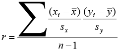
The alphabetize of biotic integrity (IBI) is a mensurate of water quality in streams. As a managing director for the natural resources in this region, you must monitor, runway, and predict changes in h2o quality. Y'all want to create a simple linear regression model that volition allow you lot to predict changes in IBI in forested expanse. The following table conveys sample data from a coastal forest region and gives the information for IBI and forested area in square kilometers. Let forest expanse exist the predictor variable (10) and IBI be the response variable (y).
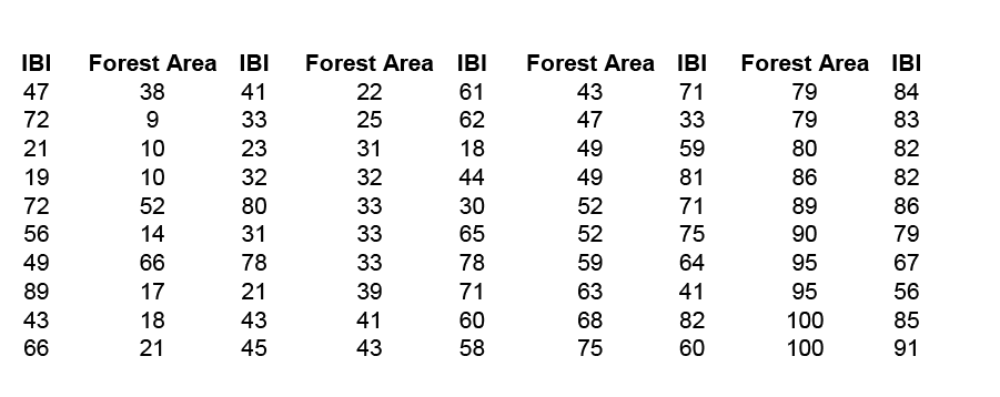
We brainstorm with a computing descriptive statistics and a scatterplot of IBI against Wood Area.
x̄ = 47.42; southwardx 27.37; ȳ = 58.80; southy = 21.38; r = 0.735
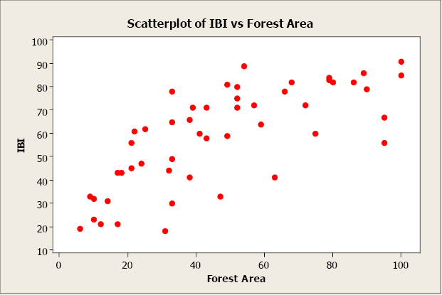
There appears to be a positive linear human relationship between the two variables. The linear correlation coefficient is r = 0.735. This indicates a strong, positive, linear relationship. In other words, wood expanse is a adept predictor of IBI. At present let'south create a elementary linear regression model using woods area to predict IBI (response).
First, we will compute b 0 and b 1 using the shortcut equations.
 =
= 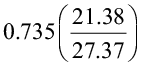 =0.574
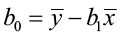
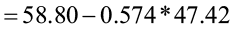 = 31.581
The regression equation is 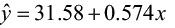 .
.
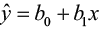
Now let's utilise Minitab to compute the regression model. The output appears below.
Regression Analysis: IBI versus Woods Area
The regression equation is IBI = 31.6 + 0.574 Wood Area
| Predictor | Coef | SE Coef | T | P |
| Constant | 31.583 | 4.177 | 7.56 | 0.000 |
| Wood Area | 0.57396 | 0.07648 | 7.50 | 0.000 |
| S = 14.6505 | R-Sq = 54.0% | R-Sq(adj) = 53.0% | ||
| Analysis of Variance | |||||
| Source | DF | SS | MS | F | P |
| Regression | 1 | 12089 | 12089 | 56.32 | 0.000 |
| Residual Error | 48 | 10303 | 215 | ||
| Full | 49 | 22392 | |||
The estimates for β 0 and β 1 are 31.half-dozen and 0.574, respectively. We can interpret the y-intercept to mean that when there is nix forested surface area, the IBI will equal 31.6. For each boosted square kilometer of forested surface area added, the IBI will increment by 0.574 units.
The coefficient of determination, R2, is 54.0%. This ways that 54% of the variation in IBI is explained by this model. Approximately 46% of the variation in IBI is due to other factors or random variation. We would like R2 to be as high as possible (maximum value of 100%).
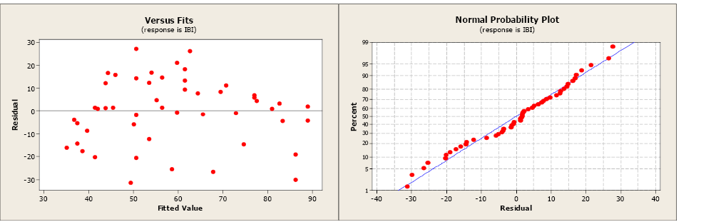
The residue and normal probability plots practise not indicate any problems.
The estimate of σ, the regression standard error, is s = 14.6505. This is a mensurate of the variation of the observed values about the population regression line. We would similar this value to be as small as possible. The MSE is equal to 215. Recall, the  = southward. The standard errors for the coefficients are 4.177 for the y-intercept and 0.07648 for the slope.
We know that the values b 0 = 31.6 and b 1 = 0.574 are sample estimates of the true, but unknown, population parameters β 0 and β 1. We can construct 95% confidence intervals to meliorate estimate these parameters. The disquisitional value (tα /ii) comes from the student t-distribution with (n – 2) degrees of freedom. Our sample size is 50 so we would accept 48 degrees of freedom. The closest tabular array value is ii.009.
95% confidence intervals for β 0 and β 1
b 0 ± tα /2 SEb0 = 31.6 ± 2.009(4.177) = (23.21, 39.99)
b 1 ± tα /2 SEb1 = 0.574 ± ii.009(0.07648) = (0.4204, 0.7277)
The next step is to exam that the slope is significantly different from zero using a 5% level of significance.
| H0: β one =0 | Hone: β i ≠0 |
t = b1 / SEb1 = 0.574/0.07648 = 7.50523
Nosotros have 48 degrees of freedom and the closest critical value from the student t-distribution is ii.009. The test statistic is greater than the critical value, then nosotros will decline the null hypothesis. The gradient is significantly different from zero. Nosotros have found a statistically pregnant relationship betwixt Wood Surface area and IBI.
The Minitab output besides report the test statistic and p-value for this test.
| The regression equation is IBI = 31.6 + 0.574 Forest Area | ||||
| Predictor | Coef | SE Coef | T | P |
| Constant | 31.583 | 4.177 | 7.56 | 0.000 |
| Wood Expanse | 0.57396 | 0.07648 | 7.fifty | 0.000 |
| S = 14.6505 | R-Sq = 54.0% | R-Sq(adj) = 53.0% | ||
| Analysis of Variance | |||||
| Source | DF | SS | MS | F | P |
| Regression | 1 | 12089 | 12089 | 56.32 | 0.000 |
| Rest Error | 48 | 10303 | 215 | ||
| Total | 49 | 22392 | |||
The t examination statistic is 7.50 with an associated p-value of 0.000. The p-value is less than the level of significance (v%) then we will turn down the cipher hypothesis. The slope is significantly dissimilar from zero. The same result can be institute from the F-exam statistic of 56.32 (7.5052 = 56.32). The p-value is the aforementioned (0.000) as the conclusion.
Conviction Interval for μ y
Now that we have created a regression model congenital on a significant relationship between the predictor variable and the response variable, we are gear up to use the model for
- estimating the average value of y for a given value of x
- predicting a particular value of y for a given value of x
Let'south examine the first choice. The sample information of n pairs that was drawn from a population was used to compute the regression coefficients b 0 and b 1 for our model, and gives us the average value of y for a specific value of ten through our population model
 . For every specific value of ten, in that location is an boilerplate y ( μ y ), which falls on the straight line equation (a line of ways). Remember, that there can be many different observed values of the y for a particular 10, and these values are causeless to have a normal distribution with a mean equal to
  and a variance of σ 2. Since the computed values of b 0 and b ane vary from sample to sample, each new sample may produce a slightly unlike regression equation. Each new model can exist used to estimate a value of y for a value of x. How far will our calculator
  be from the true population hateful for that value of ten? This depends, as e'er, on the variability in our estimator, measured past the standard error.
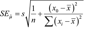
It tin exist shown that the estimated value of y when 10 = x 0 (some specified value of x), is an unbiased reckoner of the population mean, and that p̂ is unremarkably distributed with a standard mistake of
We tin construct a confidence interval to amend guess this parameter (μ y) following the aforementioned procedure illustrated previously in this chapter.
 where the disquisitional value tα /2 comes from the student t-table with (n – 2) degrees of freedom.
Statistical software, such as Minitab, volition compute the confidence intervals for you lot. Using the data from the previous case, nosotros will use Minitab to compute the 95% confidence interval for the mean response for an average forested area of 32 km.
| Predicted Values for New Observations | |||
| New Obs Fit | SE Fit | 95% | CI |
| i | 49.9496 | 2.38400 | (45.1562,54.7429) |
If you sampled many areas that averaged 32 km. of forested area, your estimate of the average IBI would be from 45.1562 to 54.7429.
Yous tin can repeat this process many times for several different values of x and plot the conviction intervals for the hateful response.
| 10 | 95% CI |
| 20 | (37.13, 48.88) |
| 40 | (l.22, 58.86) |
| sixty | (61.43, 70.61) |
| 80 | (lxx.98, 84.02) |
| 100 | (79.88, 98.07) |
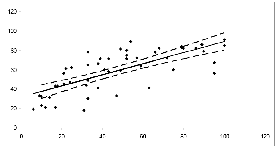
Notice how the width of the 95% confidence interval varies for the different values of x. Since the confidence interval width is narrower for the key values of x, information technology follows that μ y is estimated more precisely for values of 10 in this area. As you move towards the extreme limits of the data, the width of the intervals increases, indicating that it would exist unwise to extrapolate beyond the limits of the information used to create this model.
Prediction Intervals
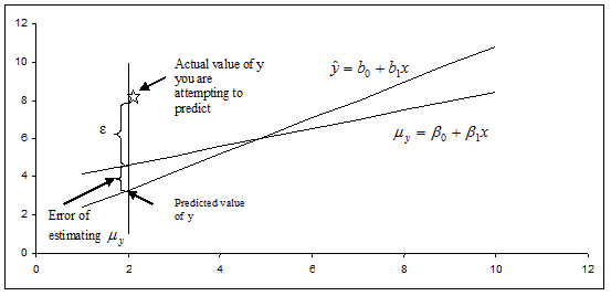
What if you lot desire to predict a particular value of y when x = x 0? Or, maybe you desire to predict the adjacent measurement for a given value of x? This trouble differs from constructing a confidence interval for μ y. Instead of amalgam a confidence interval to estimate a population parameter, we demand to construct a prediction interval. Choosing to predict a particular value of y incurs some boosted mistake in the prediction because of the deviation of y from the line of means. Examine the figure below. Yous tin encounter that the fault in prediction has two components:
- The error in using the fitted line to estimate the line of means
- The mistake acquired by the deviation of y from the line of means, measured by σ 2
The variance of the difference betwixt y and  is the sum of these ii variances and forms the basis for the standard fault of
  used for prediction. The resulting form of a prediction interval is as follows:
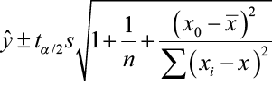
where x 0 is the given value for the predictor variable, n is the number of observations, and tα /2 is the disquisitional value with (n – ii) degrees of freedom.
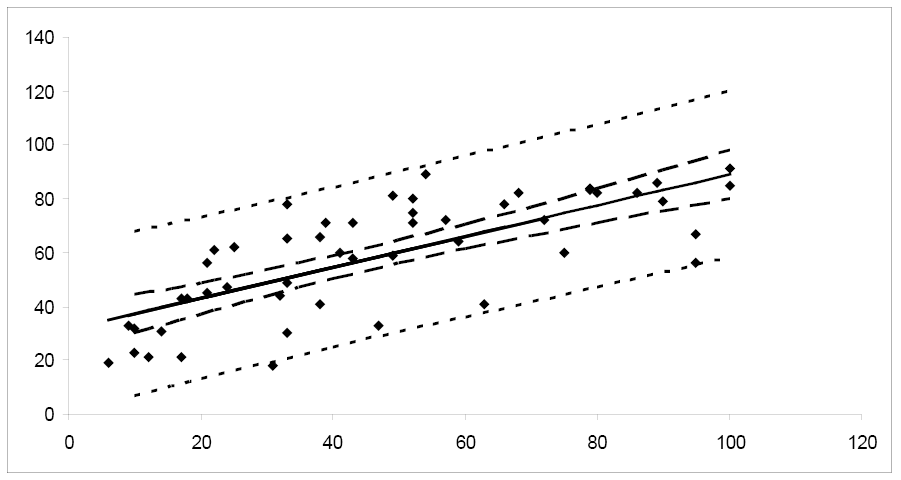
Software, such as Minitab, can compute the prediction intervals. Using the data from the previous example, nosotros will use Minitab to compute the 95% prediction interval for the IBI of a specific forested expanse of 32 km.
| Predicted Values for New Observations | |||
| New Obs | Fit | SE Fit | 95% PI |
| 1 | 49.9496 | 2.38400 | (xx.1053, 79.7939) |
You can repeat this process many times for several different values of ten and plot the prediction intervals for the hateful response.
| x | 95% PI |
| xx | (xiii.01, 73.11) |
| forty | (24.77, 84.31) |
| 60 | (36.21, 95.83) |
| 80 | (47.33, 107.67) |
| 100 | (58.15, 119.81) |
Notice that the prediction interval bands are wider than the corresponding conviction interval bands, reflecting the fact that we are predicting the value of a random variable rather than estimating a population parameter. We would expect predictions for an individual value to be more variable than estimates of an boilerplate value.
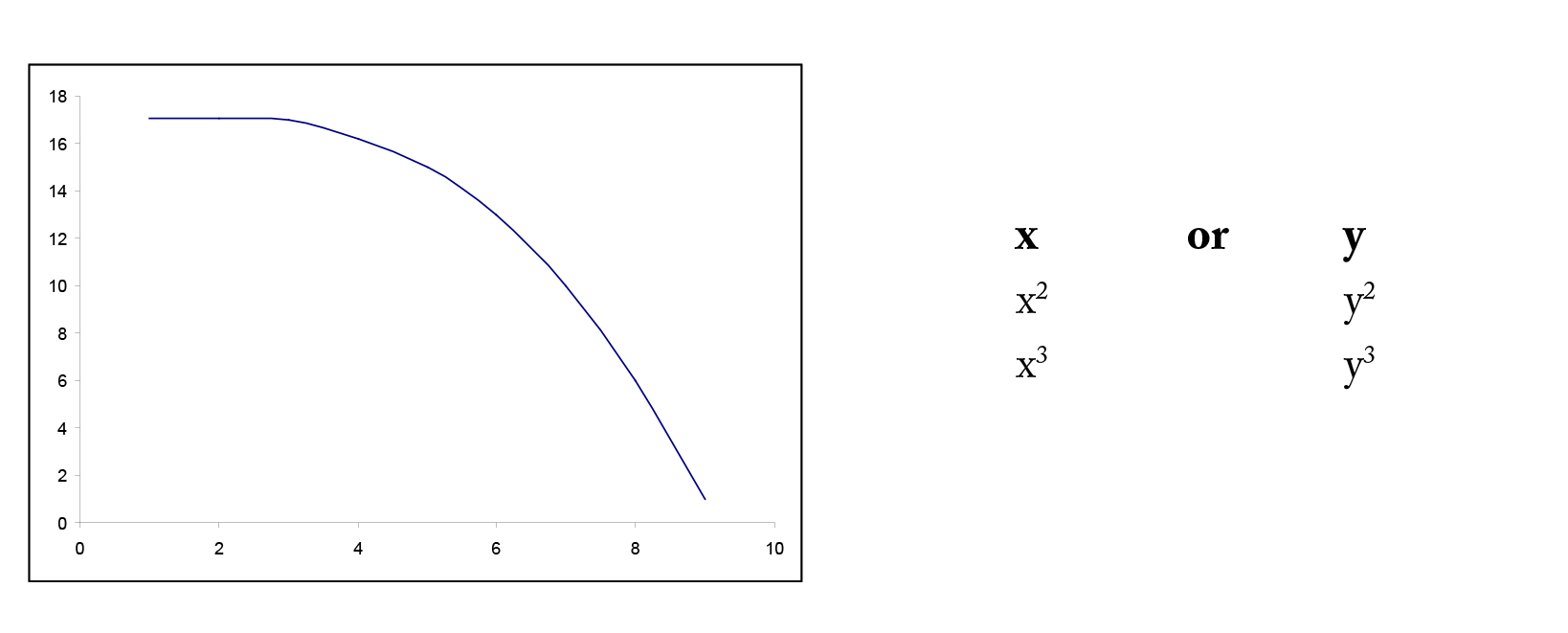
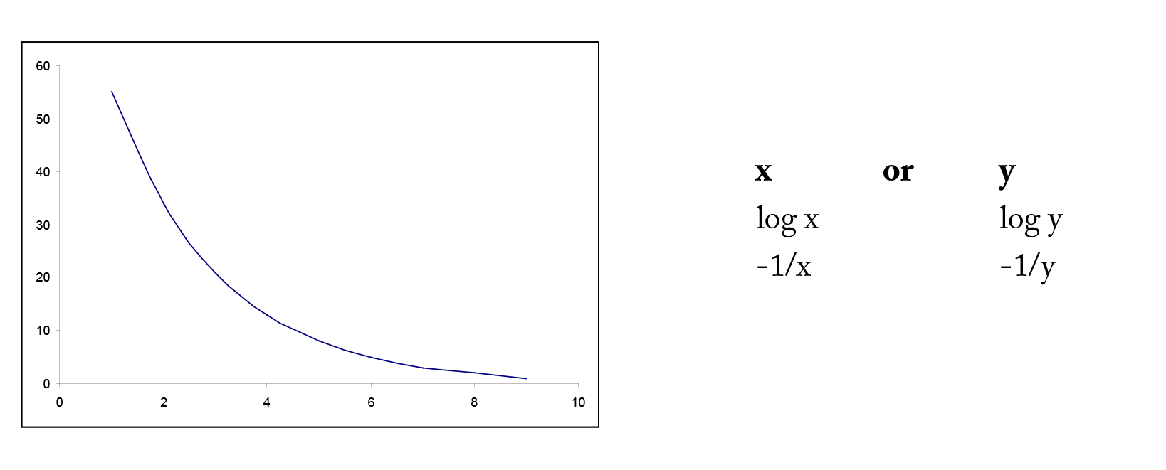
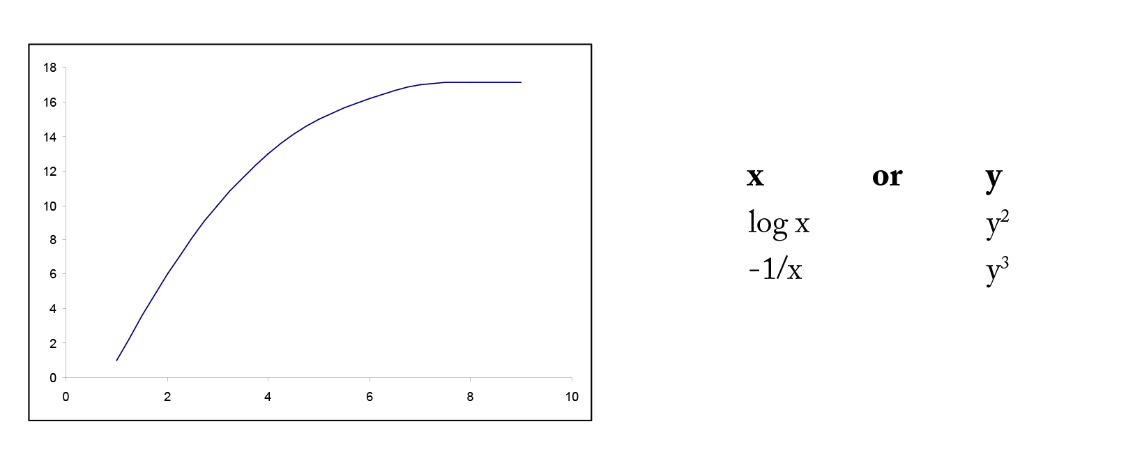
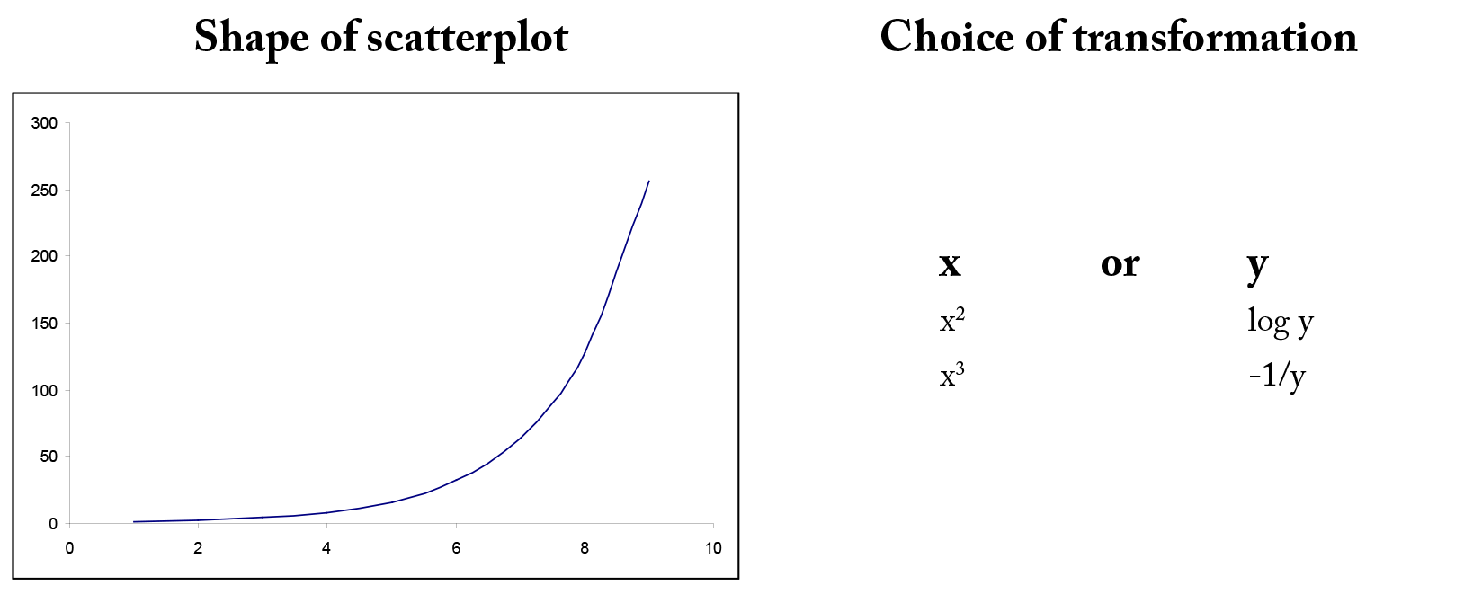
Transformations to Linearize Data Relationships
In many situations, the relationship betwixt ten and y is non-linear. In gild to simplify the underlying model, we can transform or catechumen either x or y or both to outcome in a more linear relationship. In that location are many mutual transformations such as logarithmic and reciprocal. Including higher order terms on ten may also help to linearize the relationship between x and y. Shown below are some common shapes of scatterplots and possible choices for transformations. However, the choice of transformation is ofttimes more a matter of trial and error than ready rules.
Example iv
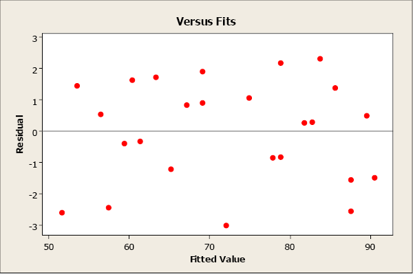
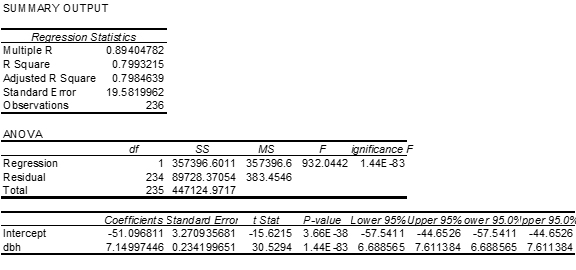
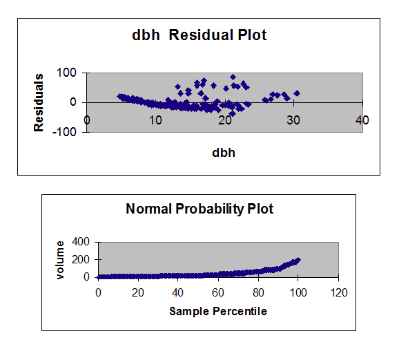
A forester needs to create a simple linear regression model to predict tree volume using diameter-at-breast height (dbh) for saccharide maple trees. He collects dbh and volume for 236 saccharide maple copse and plots volume versus dbh. Given beneath is the scatterplot, correlation coefficient, and regression output from Minitab.
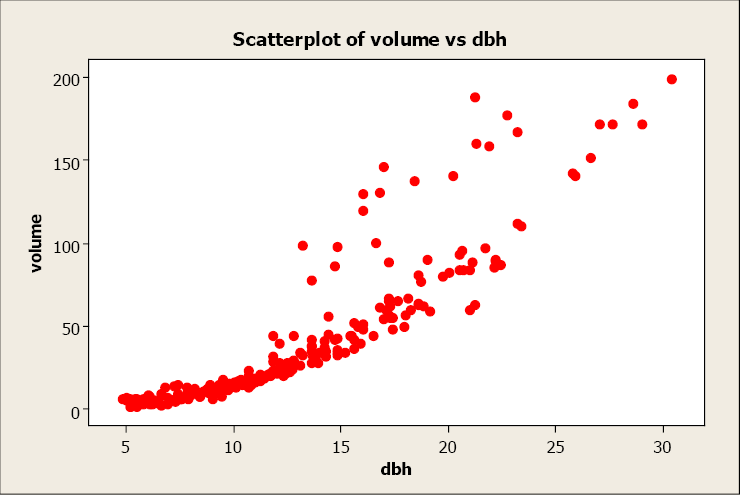
Pearson's linear correlation coefficient is 0.894, which indicates a strong, positive, linear relationship. Notwithstanding, the scatterplot shows a distinct nonlinear relationship.
Regression Analysis: volume versus dbh
| The regression equation is volume = – 51.one + seven.15 dbh | ||||
| Predictor | Coef | SE Coef | T | P |
| Constant | -51.097 | 3.271 | -15.62 | 0.000 |
| dbh | 7.1500 | 0.2342 | 30.53 | 0.000 |
| S = 19.5820 | R-Sq = 79.nine% | R-Sq(adj) = 79.eight% | ||
| Analysis of Variance | |||||
| Source | DF | SS | MS | F | P |
| Regression | 1 | 357397 | 357397 | 932.04 | 0.000 |
| Residual Error | 234 | 89728 | 383 | ||
| Total | 235 | 447125 | |||
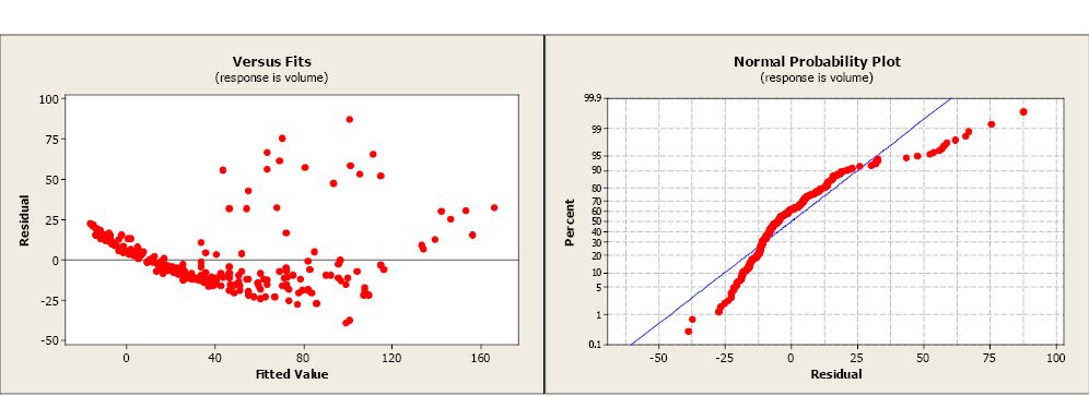
The R2 is 79.9% indicating a fairly strong model and the slope is significantly different from zero. Even so, both the residue plot and the balance normal probability plot point serious problems with this model. A transformation may help to create a more linear relationship betwixt volume and dbh.
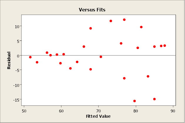
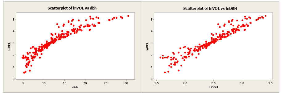
Volume was transformed to the natural log of volume and plotted against dbh (see scatterplot beneath). Unfortunately, this did little to ameliorate the linearity of this relationship. The forester so took the natural log transformation of dbh. The scatterplot of the natural log of volume versus the natural log of dbh indicated a more linear relationship between these ii variables. The linear correlation coefficient is 0.954.
The regression analysis output from Minitab is given below.
Regression Analysis: lnVOL vs. lnDBH
| The regression equation is lnVOL = – ii.86 + 2.44 lnDBH | ||||
| Predictor | Coef | SE Coef | T | P |
| Constant | -2.8571 | 0.1253 | -22.80 | 0.000 |
| lnDBH | 2.44383 | 0.05007 | 48.eighty | 0.000 |
| Southward = 0.327327 | R-Sq = 91.1% | R-Sq(adj) = 91.0% | ||
| Analysis of Variance | |||||
| Source | DF | SS | MS | F | P |
| Regression | one | 255.19 | 255.19 | 2381.78 | 0.000 |
| Residual Error | 234 | 25.07 | 0.11 | ||
| Full | 235 | 280.26 | |||
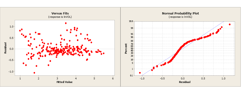
The model using the transformed values of book and dbh has a more than linear relationship and a more than positive correlation coefficient. The slope is significantly different from goose egg and the R2 has increased from 79.9% to 91.1%. The balance plot shows a more random design and the normal probability plot shows some comeback.
There are many possible transformation combinations possible to linearize data. Each state of affairs is unique and the user may demand to try several alternatives before selecting the best transformation for x or y or both.
Software Solutions
Minitab
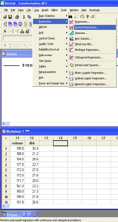
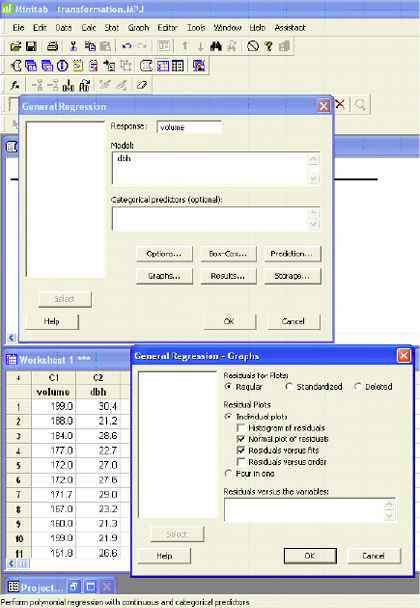
The Minitab output is shown to a higher place in Ex. 4.
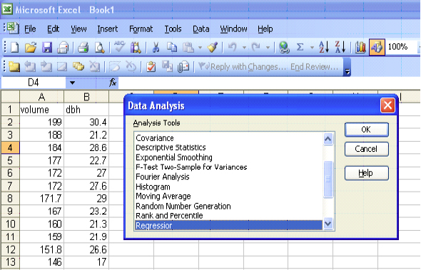
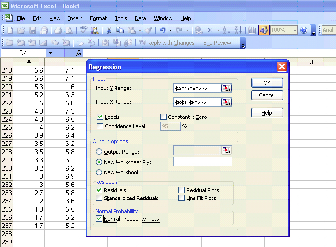
Excel

Which Regression Equation Best Fits These Data Brainly,
Source: https://milnepublishing.geneseo.edu/natural-resources-biometrics/chapter/chapter-7-correlation-and-simple-linear-regression/
Posted by: martincalloseven.blogspot.com
0 Response to "Which Regression Equation Best Fits These Data Brainly"
Post a Comment